")
Back to Journals » Infection and Drug Resistance » Volume 12
Application of a hybrid model in predicting the incidence of tuberculosis in a Chinese population
Authors Li Z , Wang Z , Song H, Liu Q , He B, Shi P, Ji Y , Xu D, Wang J
Received 10 October 2018
Accepted for publication 4 April 2019
Published 29 April 2019 Volume 2019:12 Pages 1011—1020
DOI https://doi.org/10.2147/IDR.S190418
Checked for plagiarism Yes
Review by Single anonymous peer review
Peer reviewer comments 2
Editor who approved publication: Dr Eric Nulens
Zhongqi Li,1,2 Zhizhong Wang,3 Huan Song,1 Qiao Liu,1 Biyu He,1 Peiyi Shi,1 Ye Ji,1 Dian Xu,1 Jianming Wang1,2
1Department of Epidemiology, Center for Global Health, School of Public Health, Nanjing Medical University, Nanjing, People’s Republic of China; 2Key Laboratory of Infectious Diseases, School of Public Health, Nanjing Medical University, Nanjing, People’s Republic of China; 3Department of Epidemiology and Health Statistic, School of Public Health, NingXia Medical University, Yinchuan, People’s Republic of China
Objective: To investigate suitable forecasting models for tuberculosis (TB) in a Chinese population by comparing the predictive value of the autoregressive integrated moving average (ARIMA) model and the ARIMA-generalized regression neural network (GRNN) hybrid model.
Methods: We used the monthly incidence rate of TB in Lianyungang city from January 2007 through June 2016 to construct a fitting model, and we used the incidence rate from July 2016 to December 2016 to evaluate the forecasting accuracy. The root mean square error (RMSE), mean absolute percentage error (MAPE), mean absolute error (MAE) and mean error rate (MER) were used to assess the performance of these models in fitting and forecasting the incidence of TB.
Results: The ARIMA (10, 1, 0) (0, 1, 1)12 model was selected from plausible ARIMA models, and the optimal spread value of the ARIMA-GRNN hybrid model was 0.23. For the fitting dataset, the RMSE, MAPE, MAE and MER were 0.5594, 11.5000, 0.4202 and 0.1132, respectively, for the ARIMA (10, 1, 0) (0, 1, 1)12 model, and 0.5259, 11.2181, 0.3992 and 0.1075, respectively, for the ARIMA-GRNN hybrid model. For the forecasting dataset, the RMSE, MAPE, MAE and MER were 0.2805, 8.8797, 0.2261 and 0.0851, respectively, for the ARIMA (10, 1, 0) (0, 1, 1)12 model, and 0.2553, 5.7222, 0.1519 and 0.0571, respectively, for the ARIMA-GRNN hybrid model.
Conclusions: The ARIMA-GRNN hybrid model was shown to be superior to the single ARIMA model in predicting the short-term TB incidence in the Chinese population, especially in fitting and forecasting the peak and trough incidence.
Keywords: model, ARIMA, GRNN, tuberculosis, incidence, forecasting
Introduction
Tuberculosis (TB) is an ancient infectious disease that is caused by Mycobacterium tuberculosis (M.tb), and pulmonary tuberculosis is the most common type. According to the Global tuberculosis report 2018, there were approximately 10 million new cases and 1.57 million deaths due to TB in 2017. Globally, TB is the tenth leading cause of death and is the leading cause of death from a single infectious agent.1 Although the global TB incidence is declining at a rate of 2% per year, there is still a long way to go to reach the first milestone of the “End TB” strategy, due to the challenges of multidrug-resistant TB (MDR-TB), TB-HIV dual infection and high incidence of TB in the floating population.2–4 By collecting long-term TB morbidity data and selecting appropriate models, it is possible to predict the trend of TB epidemics, thereby anticipating possible outbreaks and guiding emergency preparedness at an early stage.
The autoregressive integrated moving average (ARIMA) model, which is also known as the Box-Jenkins model, was proposed by George Box and Gwilym Jenkins in the early 1970s. The ARIMA model assigns the combined effects of multiple risk factors that affect the disease occurrence and prevalence to time. This model has become one of the most popular and convenient models in time series analysis, and it has been widely used in the prediction of infectious diseases, such as malaria,5–9 influenza,10–13 hand-foot-mouth disease (HMFD),14–16 hepatitis,17 dengue fever18 and hemorrhagic fever.19 Nevertheless, the ARIMA model has a limitation of preassumed linearity, which often does not conform to real-world problems, as the incidence of infectious diseases is affected by a variety of uncertain factors and usually exhibits nonlinear characteristics.20,21 Another commonly used model is the generalized regression neural network (GRNN). This model belongs to the artificial neural network (ANN) family, and its advantages include a small sample size, few parameters for artificial determination and strong nonlinear fitting ability. In recent years, the GRNN model has performed well in predicting epidemics either solely22 or in combination with the ARIMA model.23,24
The ARIMA model has been used previously to predict the incidence of TB,25–27 but the GRNN model and the ARIMA-GRNN hybrid model have rarely been studied. In the current study, we collected surveillance data of TB in a Chinese population and compared the predictive value of the ARIMA model and the ARIMA-GRNN hybrid model with the aim of providing a tool for decision making in the early warning system for managing TB.
Materials and methods
Study area and data collection
We selected Lianyungang as the study site. This city is located in the northeastern part of Jiangsu province in China with an area of approximately 7.6 thousand square kilometers and a permanent population of 4.52 million in 2017. Surveillance data of TB from January 2007 to December 2016 were extracted from the Lianyungang Center for Disease Control and Prevention (CDC). Population data were obtained from the Lianyungang Statistical Yearbook. We used the incidence data from January 2007 to June 2016 as the model-constructing dataset and the incidence data from July 2016 to December 2016 as the model-validating dataset.
Construction of ARIMA model
The ARIMA model is written in shorthand as ARIMA (p, d, q) (P, D, Q)s, where p, d and q represent the autoregressive order, the number of nonseasonal differences and the moving average order, respectively, and P, D and Q represent the seasonal autoregressive order, the number of seasonal differences and the seasonal moving average order, respectively, and s indicates the length of the cyclical pattern. The construction of the ARIMA model included the following four steps: First, we determined that the series was nonstationary from the incidence series plot, which exhibited a long-term trend and seasonal fluctuations. The existence of a long-term trend was also demonstrated by the Mann-Kendall trend test. We applied one nonseasonal difference and one seasonal difference to stabilize the series, and the series was confirmed to be stationary through the difference analysis according to the Augmented Dickey–Fuller (ADF) test. Second, we identified optional parameters (p and q, P and Q) to establish one or more alternative models by referring to the autocorrelation function (ACF) and partial autocorrelation function (PACF) plots of the stationary series. We first determined the parameters of the seasonal part of the ARIMA model (P and Q) and then defined the parameters of the nonseasonal part (p and q). The model with the lowest corrected Akaike’s information criterion (AICc) and Bayesian information criterion (BIC) was regarded as the optimal model. Third, we used the maximum likelihood method to estimate the parameters and the Ljung-Box test to examine the residual series of the optimal model. The residual series should be white noise, demonstrating that the model completely extracted the information from the original data. Moreover, the ACF and PACF plots of the residual series should not show any significant correlation. Finally, the optimal model was applied to predict the TB incidence and compare this prediction with the validating dataset.12,16,19
ARIMA-GRNN hybrid model
The GRNN, which is a branch of the artificial neural network (ANN), is a feedforward neural network based on the nonlinear regression theory. This network examines the relationship between each pair of the input vector  and the observed output
  and finally deduces the inherent function, which can be summarized with the following equation:
 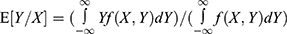 , where
  is the input vector
  and
and  is the predicted vector
  of GRNN.
  is the expected value of the output
  with a given input vector
  , and
, and  is the joint probability density of
  and
and  .
.
The structure of GRNN consists of the following four layers: the input layer, pattern layer, summation layer and output layer. The number of neurons in the input layer is equal to the dimension of the input vector in the learning samples. Each neuron in the input layer is a simple distribution unit that can directly submit the input variables to the pattern layer. The number of neurons in the pattern layer is equal to the number of learning samples, and each neuron corresponds to a different sample. The transfer function of neurons of the pattern layer is calculated with the following equation: 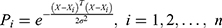 , where
  is the output of the neurons in the pattern layer;
 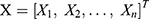 is the input vector;
  is the learning samples of the
  -th neurons;
  is the number of input;
  is the number of neurons; and
  is the spread factor. There are two types of summation for the neurons of the summation layer. One type of summation is to arithmetically sum the output of neurons of the pattern layer. The connection weight between the pattern layer and each neuron is 1. The formula of the transfer function is as follows:
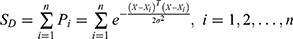 . The other type of summation is to sum the weighted output of neurons of the pattern layer. The connection weight between the
  -th neuron of the pattern layer and the
  -th summation neuron is equal to the
  -th element in the
  -th output samples of
  The formula of transfer function is as follows:
 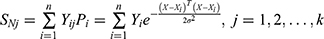 , where
  is the dimension of the output vector. The number of neurons of the output layer and the dimension of the input vector of the learning samples are the same. The formula of the output of the
  -th neurons is as follows:
 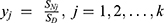 .28
.28
In contrast to the traditional error back propagation algorithm, the learning algorithm of GRNN does not need to adjust for the connection weight between neurons during the training process; rather, the GRNN changes the spread factor to adjust for the transfer function of each unit to obtain the best regression estimation result. The spread factor has a strong influence on the prediction performance of the network. A smaller spread factor leads to a stronger approximation performance of the network to the sampling data; in contrast, a larger spread factor leads to a smoother approximation process of the network to the sampling data.
The estimated values of the ARIMA model are usually different from the actual values, since the ARIMA model is designed to analyze the liner part of the original data, and the residual series from this linear model will contain a nonlinear relationship.24 The ARIMA model excels at extracting linear information from original data, while the GRNN model has strong advantages in nonlinear fitting models, which can make up for the shortcomings of the ARIMA model. The ARIMA-GRNN hybrid model combines the advantages of these two models and can therefore thoroughly exploit data information. We used the fitting data from the ARIMA model as the input values and the actual data as the output values to construct the GRNN model. Through the process of GRNN learning and simulating data repeatedly, the association between the fitting data of the ARIMA model and the actual data can be evaluated effectively, and the nonlinear component of the latter can be obtained. Therefore, the actual contribution of this hybrid model is that it can correct the fitting and predicting values of the ARIMA model so that the corrected values are more in line with the actual values. We determined the spread factor according to the method proposed by Specht. Two months were randomly selected as the testing samples to determine the optimal spread value. We let the spread value increase incrementally within a certain range, and then we calculated the root mean square error (RMSE) between the output incidence and the actual incidence of the two testing samples. The minimum RMSE value corresponded to the optimal spread value.24,29,30 Once the optimal spread value was identified, we used the forecasting incidence of the ARIMA model as the input values and applied the trained GRNN model to predict the future TB incidence.
Comparison of the two models
The indices including RMSE, mean absolute percentage error (MAPE), mean absolute error (MAE) and mean error rate (MER) were used to evaluate the performance of the models in fitting and forecasting the TB incidence in the study site. 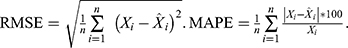
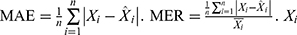 is the actual incidence at time
  ,
,  is the fitting or forecasting incidence at time
  ,
,  is the mean of the actual incidence, and
  is the number of samples.
Statistical software
We used the packages of “forecast,” “ggplot2,” “trend” and “tseries” of R3.5.1 (
Ethics statement
This study was approved by the Ethics Committee of Nanjing Medical University. After informed consent was obtained from all participants, questionnaires were used to collect demographic data.
Results
Construction of the ARIMA model
The monthly TB incidence during January 2007 and June 2016 in Lianyungang is shown in Figure 1. Based on the incidence series plot, we observed a slight declining trend (P <0.001) and seasonal fluctuations (s =12). The peak incidence primarily occurred in March, April, May, November and December. The trough was more common in January and February. We applied both nonseasonal (d =1) difference and seasonal difference (D =1) to eliminate numerical instabilities. The plot of the original incidence series after one nonseasonal and one seasonal difference is shown in File S1, from which we preliminarily judged that the declining trend and seasonal fluctuations were eliminated. The ADF test remained significant (P <0.001) after the nonseasonal and seasonal difference, indicating a stationary incidence series. The declining trend proved to be eliminated by the nonseasonal difference according to the Mann-Kendall trend test (P =0.85). The seasonal fluctuations were demonstrated to be eliminated by the seasonal difference according to the ACF and PACF plots; only lag 12 exhibited a significant spike in the ACF plot, whereas lag 12 and 24 exhibited no significant spikes in the PACF plot (Figure 2A). For the seasonal part of the ARIMA model, there was a significant spike at lag 12 in the ACF plot, but there was no significant spike at lag 24 (Q =1) in the ACF plot or at lag 12 or 24 in the PACF plot (P =0). For the nonseasonal part of the ARIMA model, in the first cycle, there were three significant spikes (lag 1, lag 10 and lag 11) in the ACF plot and four significant spikes (lag 1, lag 2, lag 10 and lag 11) in the PACF plot. We initially considered the following nine possibilities: p =0 and q =1; p =1 and q =0; p =1 and q =1; p =2 and q =0; p =2 and q =1; p =10 and q =0; p =11 and q =0; p =0 and q =10; p =0 and q =11, since the ACF and PACF plots did not show an obvious pattern. The AICc and BIC values and the Ljung-Box test results of residual series of these nine plausible ARIMA models are listed in Table 1. We selected ARIMA (10,1,0) (0,1,1)12 as the optimal model, as this model had resulted in the minimum AICc and BIC values, indicating that the residual series represented white noise. The parameter estimation of this model is shown in Table 2. The ACF and PACF plots of residual series were also demonstrated to be white noise, since their correlation coefficients were not beyond the confidence borders (Figure 2B). Then, we applied the ARIMA (10,1,0) (0,1,1)12 model to predict the TB incidence during July 2016 and December 2016. The predictive data are listed in Table 3.
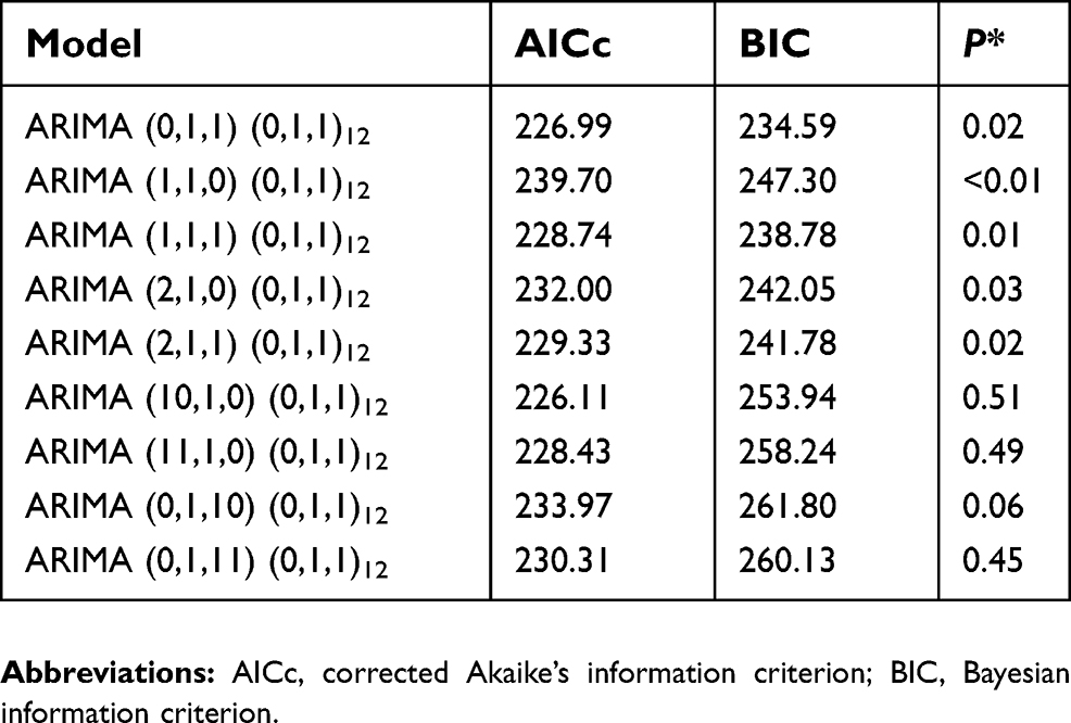 | Table 1 AICc and BIC values and the Ljung-Box test results of residual series of plausible ARIMA models |
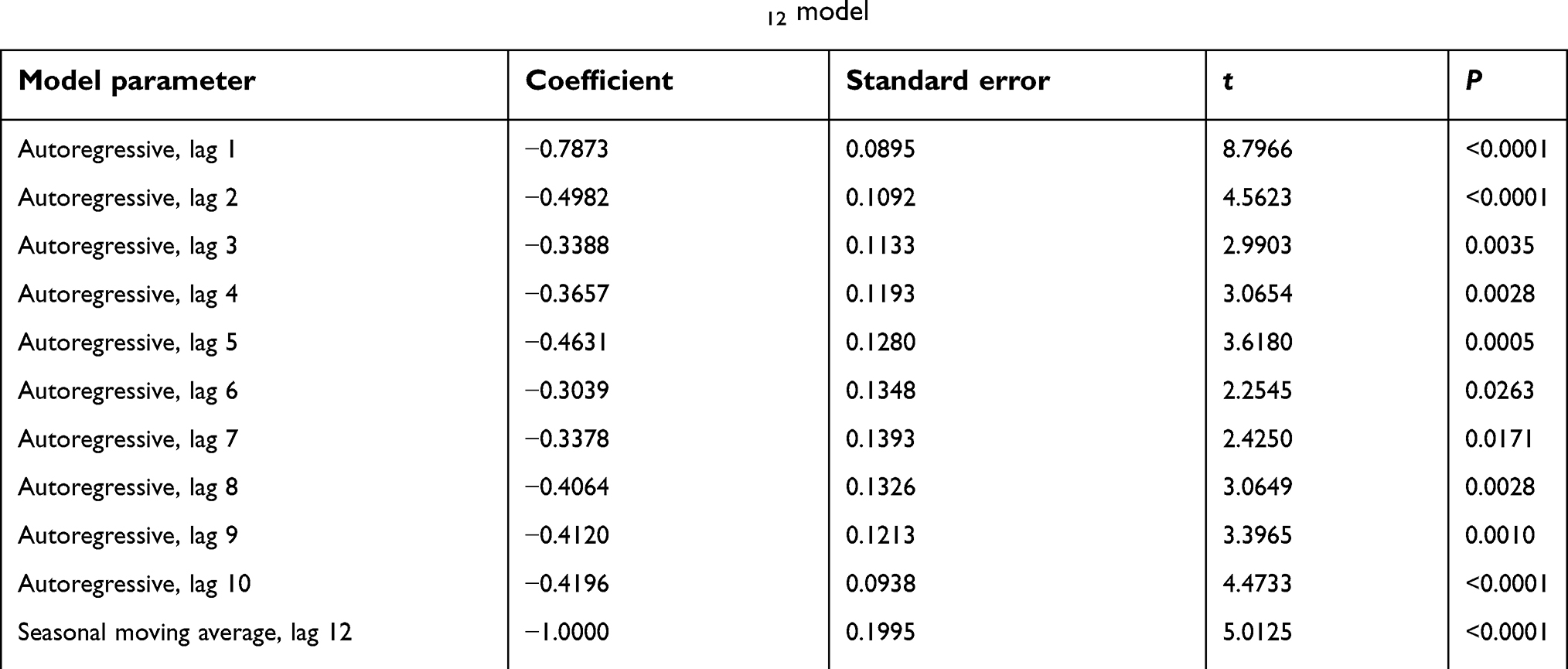 | Table 2 Estimation of parameters of the ARIMA (10,1,0) (0,1,1)12 model |
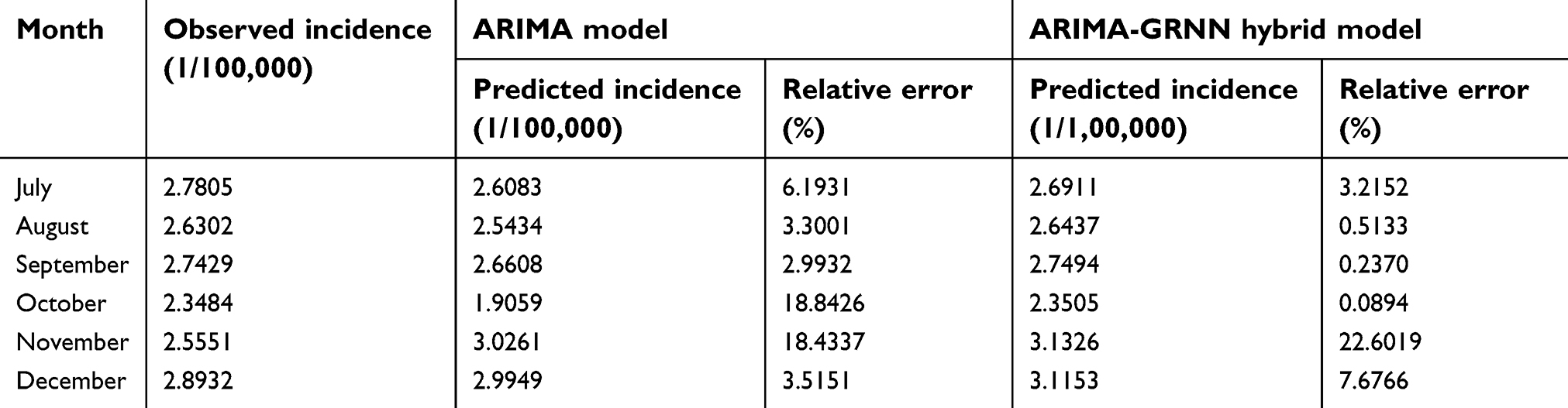 | Table 3 Predicted TB incidence by the ARIMA and ARIMA-GRNN hybrid models from July to December 2016 |
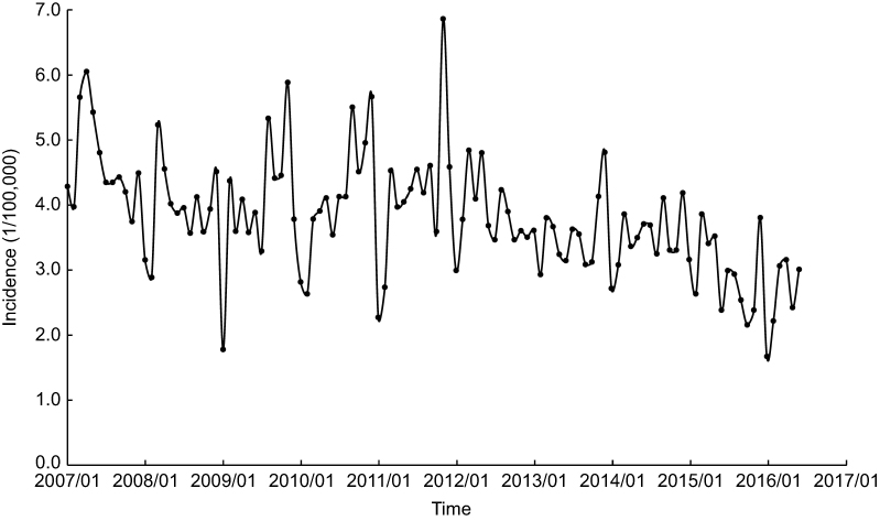 | Figure 1 Monthly reported TB incidence from January 2007 to June 2016 in Lianyungang. |
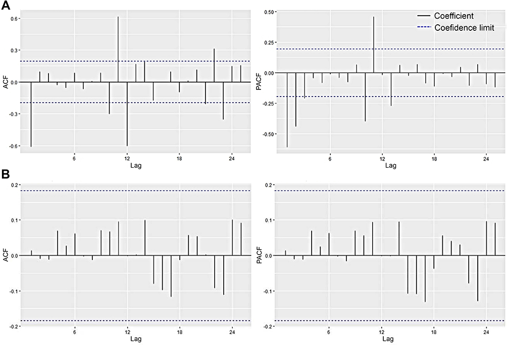 | Figure 2 ACF and PACF plots. (A): The ACF and PACF plots of TB incidence series after the application of one nonseasonal difference and one seasonal difference; (B): The ACF and PACF plots of residual series of the ARIMA (10,1,0) (0,1,1)12 model.Abbreviations: ACF, autocorrelation function; PACF, partial autocorrelation function. |
Construction of the ARIMA-GRNN hybrid model
Due to the one nonseasonal difference and one seasonal difference, the information of thirteen months was lost in the construction of the ARIMA-GRNN hybrid model. The fitting incidence of the ARIMA model and the actual incidence between February 2008 and June 2016 were used as the input and output values of the GRNN model, respectively. We randomly selected data in March 2008 and January 2014 as the testing samples to determine the optimal spread value. We observed that the spread value gradually increased from 0.01 to 0.5 with an interval of 0.01; the corresponding RMSE values between the output and actual incidence of the two testing samples are shown in Figure 3. Since the RMSE reached the minimum value when the spread value was 0.23, we set the optimal spread value as 0.23. Eventually, we used the predicted incidence of ARIMA model as the input values and applied the trained GRNN model to predict the incidence of TB from July 2016 to December 2016 (Table 3).
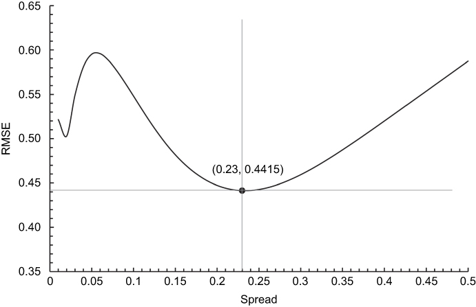 | Figure 3 Selection of the optimal spread value for the ARIMA-GRNN hybrid model. |
Comparison of the two models
The performance of the single ARIMA model and the ARIMA-GRNN hybrid model in fitting and forecasting TB incidence was compared based on the RMSE, MAPE, MAE and MER (Table 4). Although the hybrid model was slightly inferior to the single ARIMA model in forecasting the TB incidence of the last two months in 2016, generally speaking, the hybrid model performed better. As shown in Figure 4, the hybrid model was more accurate than the single ARIMA model, especially in terms of fitting and forecasting the peak and trough incidence.
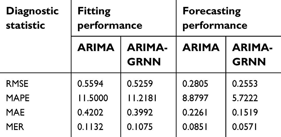 | Table 4 Comparison of the fitting and forecasting performance of the ARIMA and ARIMA-GRNN hybrid models |
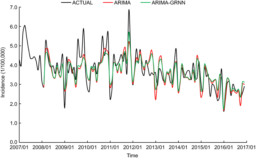 | Figure 4 Fitting and forecasting curves of the ARIMA and ARIMA-GRNN hybrid models and the actual reported TB incidence. |
Discussion
Although the incidence of TB has declined in recent years, China is still one of the thirty countries with the highest TB burden.1,3 Accurately predicting the incidence of TB is essential for policy-makers to make effective interventions in a timely manner and to allocate health resources reasonably. The early detection of the peak incidence is conducive to raising awareness. In this study, we used the incidence data of TB in a Chinese population to construct a predictive model, and we observed that the ARIMA-GRNN hybrid model was superior to the single ARIMA model. These findings indicate the potential value of the hybrid model in forecasting the short-term TB incidence in the study area.
TB incidence in the study site exhibited a downward trend from 2007 to 2016, which may be attributed to the government’s commitment to controlling TB, an increased budget and an improved public health system.23 We observed distinct seasonal fluctuations in the incidence of TB in this area. In contrast to certain areas that have one peak of incidence in the spring, this study site showed another peak in late autumn and early winter.3 Different seasonal characteristics of the TB incidence can be observed in different areas. For example, studies in Japan and Spain showed that spring was the season with a higher TB incidence,31,32 whereas in the UK, the incidence peak was in the summer.33
The ARIMA model is a combination of an autoregressive model and a moving average model, which can analyze both nonseasonal and seasonal time series. After logarithmic transformation and/or difference adjustment, even nonstationary time series can also be analyzed by the ARIMA model, which accounts for the capacity of this model to forecast disease. For example, Liu et al used the ARIMA (1,0,1) (0,1,0)12 model to predict the HFMD incidence in Sichuan province, China.16 Wangdi et al used the ARIMA (2,1,1) (0,1,1)12 model to predict malaria in endemic districts of Bhutan.5 Wang et al used the ARIMA (1,1,1) (1,1,0)12 model to predict influenza morbidity in Ningbo, China.11 Although the ARIMA model has a relative high prediction accuracy, it has limitations in processing nonlinear data.24 Alternatively, the GRNN model can make up for this disadvantage because of its powerful nonlinear fitting ability. The GRNN model is a specific form of radial basis function neural networks (RBFNN). First, the model’s network structure is relatively simple, including only two hidden layers (the pattern layer and the summation layer). Second, the model’s network training is notably easy. When the training samples pass through the hidden layer, the network training has already been completed, which avoids a long training time and high computational cost. Third, because of the simple network structure, it is not necessary to estimate or guess the number of hidden layers and hidden units of the network. In addition, only one free parameter (the spread) needs to be determined, which is the smoothing parameter of the RBF.20,23
The occurrence of tuberculosis is usually affected by various factors, and it is often difficult to identify all the characteristics of the disease sequence.34,35 Simply using the linear or nonlinear model cannot extract adequate information. In the current study, we observed that the ARIMA-GRNN hybrid model has a higher prediction accuracy compared with the single ARIMA model, which is consistent with previous studies.3,20,23,24 Since the construction of the ARIMA-GRNN hybrid model is based on the ARIMA model, its prediction accuracy is affected by the performance of the ARIMA model. Adding more variables that affect TB transmission into the model can improve the accuracy of prediction models.35 Additionally, it is noteworthy that the ARIMA-based model is a short-term prediction model, and its application to predicting long-term trends needs to be performed with caution. In addition, the application value of this hybrid model needs to be demonstrated in additional studies in other areas.
In conclusion, the ARIMA-GRNN hybrid model was shown to be superior to the single ARIMA model in predicting the short-term TB incidence, especially in fitting and forecasting the peak and trough incidence.
Acknowledgments
This work was supported by the National Key R&D Program of China (2017YFC0907000), National Natural Science Foundation of China (81473027) and the Priority Academic Program Development of Jiangsu Higher Education Institutions (PAPD). The funders had no role in the study design, data collection and analysis, decision to publish, or preparation of the manuscript.
Author contributions
All authors contributed to data analysis, drafting or revising the article, gave final approval of the version to be published, and agree to be accountable for all aspects of the work.
Disclosure
The authors report no conflicts of interest in this work.
References
1.
2. Sgaragli G, Frosini M. Human tuberculosis I. Epidemiology, diagnosis and pathogenetic mechanisms. Curr Med Chem. 2016;23(25):2836–2873.
3. Wang H, Tian CW, Wang WM, Luo XM. Time-series analysis of tuberculosis from 2005 to 2017 in China. Epidemiol Infect. 2018;146(8):935–939. doi:10.1017/S0950268818001115
4. Lv L, Li T, Xu K, et al. Sputum bacteriology conversion and treatment outcome of patients with multidrug-resistant tuberculosis. Infect Drug Resist. 2018;11:147–154. doi:10.2147/IDR.S153499
5. Wangdi K, Singhasivanon P, Silawan T, Lawpoolsri S, White NJ, Kaewkungwal J. Development of temporal modelling for forecasting and prediction of malaria infections using time-series and ARIMAX analyses: a case study in endemic districts of Bhutan. Malar J. 2010;9(1):251. doi:10.1186/1475-2875-9-251
6. Ramirez AP, Buitrago JI, Gonzalez JP, Morales AH, Carrasquilla G. Frequency and tendency of malaria in Colombia, 1990 to 2011: a descriptive study. Malar J. 2014;13(1):202. doi:10.1186/1475-2875-13-202
7. Briet OJ, Amerasinghe PH, Vounatsou P. Generalized seasonal autoregressive integrated moving average models for count data with application to malaria time series with low case numbers. PLoS One. 2013;8(6):e65761. doi:10.1371/journal.pone.0065761
8. Briet OJ, Vounatsou P, Gunawardena DM, Galappaththy GN, Amerasinghe PH. Models for short term malaria prediction in Sri Lanka. Malar J. 2008;7(1):76. doi:10.1186/1475-2875-7-129
9. Anwar MY, Lewnard JA, Parikh S, Pitzer VE. Time series analysis of malaria in Afghanistan: using ARIMA models to predict future trends in incidence. Malar J. 2016;15(1):566. doi:10.1186/s12936-016-1602-1
10. N‘Gattia AK, Coulibaly D, Nzussouo NT, et al. Effects of climatological parameters in modeling and forecasting seasonal influenza transmission in Abidjan, Cote d‘Ivoire. BMC Public Health. 2016;16(1):972. doi:10.1186/s12889-016-3503-1
11. Wang C, Li Y, Feng W, et al. Epidemiological features and forecast model analysis for the morbidity of influenza in Ningbo, China, 2006–2014. Int J Environ Res Public Health. 2017;14(6):559. doi:10.3390/ijerph14060559
12. Chadsuthi S, Iamsirithaworn S, Triampo W, Modchang C. Modeling seasonal influenza transmission and its association with climate factors in thailand using time-series and ARIMAX analyses. Comput Math Methods Med. 2015;2015:436495. doi:10.1155/2015/436495
13. Song X, Xiao J, Deng J, Kang Q, Zhang Y, Xu J. Time series analysis of influenza incidence in Chinese provinces from 2004 to 2011. Medicine (Baltimore). 2016;95(26):e3929. doi:10.1097/MD.0000000000004864
14. Yu L, Zhou L, Tan L, et al. Application of a new hybrid model with seasonal auto-regressive integrated moving average (ARIMA) and nonlinear auto-regressive neural network (NARNN) in forecasting incidence cases of HFMD in Shenzhen, China. PLoS One. 2014;9(6):e98241. doi:10.1371/journal.pone.0098241
15. Du Z, Xu L, Zhang W, Zhang D, Yu S, Hao Y. Predicting the hand, foot, and mouth disease incidence using search engine query data and climate variables: an ecological study in Guangdong, China. BMJ Open. 2017;7(10):e016263. doi:10.1136/bmjopen-2017-016263
16. Liu L, Luan RS, Yin F, Zhu XP, Lu Q. Predicting the incidence of hand, foot and mouth disease in Sichuan province, China using the ARIMA model. Epidemiol Infect. 2016;144(1):144–151. doi:10.1017/S0950268815001144
17. Ren H, Li J, Yuan ZA, Hu JY, Yu Y, Lu YH. The development of a combined mathematical model to forecast the incidence of hepatitis E in Shanghai, China. BMC Infect Dis. 2013;13(1):421. doi:10.1186/1471-2334-13-421
18. Mekparyup J, Saithanu K. A new approach to detect epidemic of DHF by combining ARIMA model and adjusted Tukey‘s control chart with interpretation rules. Interv Med Appl Sci. 2016;8(3):118–120. doi:10.1556/1646.8.2016.3.6
19. Wang T, Liu J, Zhou Y, et al. Prevalence of hemorrhagic fever with renal syndrome in Yiyuan county, China, 2005–2014. BMC Infect Dis. 2016;16(1):69. doi:10.1186/s12879-016-1987-z
20. Wei W, Jiang J, Liang H, et al. Application of a combined model with Autoregressive Integrated Moving Average (ARIMA) and Generalized Regression Neural Network (GRNN) in forecasting hepatitis incidence in Heng County, China. PLoS One. 2016;11(6):e0156768. doi:10.1371/journal.pone.0156768
21. Wu W, Guo J, An S, et al. Comparison of two hybrid models for forecasting the incidence of hemorrhagic fever with renal syndrome in Jiangsu province, China. PLoS One. 2015;10(8):e0135492. doi:10.1371/journal.pone.0135492
22. El-Solh AA, Hsiao C-B, Goodnough S, Serghani J, Grant BJB. Predicting active pulmonary tuberculosis using an artificial neural network. Chest. 1999;116(4):968–973.
23. Zhang G, Huang S, Duan Q, et al. Application of a hybrid model for predicting the incidence of tuberculosis in Hubei, China. PLoS One. 2013;8(11):e80969. doi:10.1371/journal.pone.0080969
24. Yan W, Xu Y, Yang X, Zhou Y. A hybrid model for short-term bacillary dysentery prediction in Yichang City, China. Jpn J Infect Dis. 2010;63(4):264–270.
25. Permanasari AE, Rambli DR, Dominic PD. Performance of univariate forecasting on seasonal diseases: the case of tuberculosis. Adv Exp Med Biol. 2011;696(696):171–179. doi:10.1007/978-1-4419-7046-6_17
26. Li XX, Wang LX, Zhang H, et al. Seasonal variations in notification of active tuberculosis cases in China, 2005–2012. PLoS One. 2013;8(7):e68102. doi:10.1371/journal.pone.0068102
27. Wubuli A, Li Y, Xue F, et al. Seasonality of active tuberculosis notification from 2005 to 2014 in Xinjiang, China. PLoS One. 2017;12(7):e0180226. doi:10.1371/journal.pone.0180226
28. Gan R, Chen N, Huang D. Comparisons of forecasting for hepatitis in Guangxi Province, China by using three neural networks models. PeerJ. 2016;4(2):e2684. doi:10.7717/peerj.2684
29. Specht DF. A general regression neural network. IEEE Trans Neural Netw. 1991;2(6):568–576. doi:10.1109/72.97934
30. He F, Hu ZJ, Zhang WC, Cai L, Cai GX, Aoyagi K. Construction and evaluation of two computational models for predicting the incidence of influenza in Nagasaki Prefecture, Japan. Sci Rep. 2017;7(1):7192. doi:10.1038/s41598-017-07475-3
31. Nagayama N, Ohmori M. Seasonality in various forms of tuberculosis. Int J Tuberc Lung Dis. 2006;10(10):1117–1122.
32. Rios M, Garcia JM, Sanchez JA, Perez D. A statistical analysis of the seasonality in pulmonary tuberculosis. Eur J Epidemiol. 2000;16(5):483–488.
33. Douglas AS, Strachan DP, Maxwell JD. Seasonality of tuberculosis: the reverse of other respiratory diseases in the UK. Thorax. 1996;51(9):944–946.
34. Wang M, Kong W, He B, et al. Vitamin D and the promoter methylation of its metabolic pathway genes in association with the risk and prognosis of tuberculosis. Clin Epigenetics. 2018;10(1):118. doi:10.1186/s13148-018-0552-6
35. Xu G, Mao X, Wang J, Pan H. Clustering and recent transmission of mycobacterium tuberculosis in a Chinese population. Infect Drug Resist. 2018;11:323–330. doi:10.2147/IDR.S156534
Supplementary material
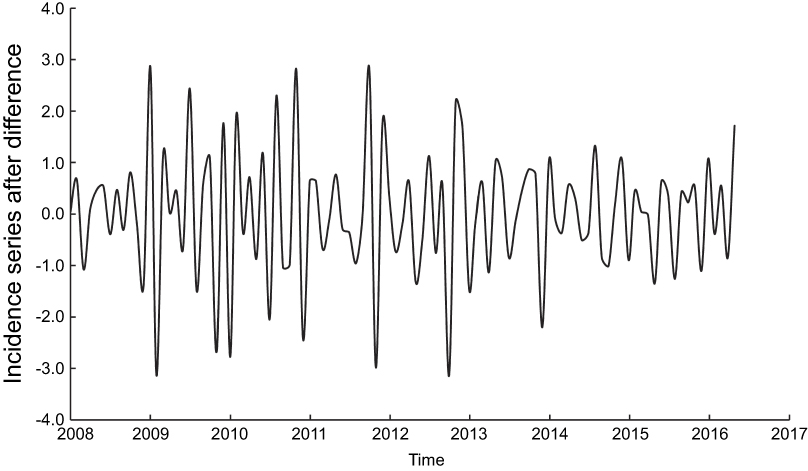 | Figure S1. Incidence series after the application of one nonseasonal difference and one seasonal difference. |
 © 2019 The Author(s). This work is published and licensed by Dove Medical Press Limited. The full terms of this license are available at https://www.dovepress.com/terms.php and incorporate the Creative Commons Attribution - Non Commercial (unported, v3.0) License.
By accessing the work you hereby accept the Terms. Non-commercial uses of the work are permitted without any further permission from Dove Medical Press Limited, provided the work is properly attributed. For permission for commercial use of this work, please see paragraphs 4.2 and 5 of our Terms.
© 2019 The Author(s). This work is published and licensed by Dove Medical Press Limited. The full terms of this license are available at https://www.dovepress.com/terms.php and incorporate the Creative Commons Attribution - Non Commercial (unported, v3.0) License.
By accessing the work you hereby accept the Terms. Non-commercial uses of the work are permitted without any further permission from Dove Medical Press Limited, provided the work is properly attributed. For permission for commercial use of this work, please see paragraphs 4.2 and 5 of our Terms.